Determination of g, K and I
Using a Compound Pendulum
A polished interactive lab workspace covering theory, apparatus, procedure, simulation, observations, and result analysis for this undergraduate experiment.
Objective
Section 01Aim
Determination of Acceleration Due to Gravity (g), Radius of Gyration (K), and Moment of Inertia (I) of a Bar Using a Compound Pendulum.
Learning Objectives
After completing this experiment, students will be able to:
- Understand the principle and construction of a compound pendulum.
- Measure the time period of oscillation for different points of suspension.
- Study the variation of the time period with the distance of the point of suspension from the centre of gravity.
- Determine the equivalent length of the compound pendulum.
- Determine the acceleration due to gravity (g) using experimental observations.
- Determine the radius of gyration (K) and moment of inertia (I) of the pendulum.
- Plot and interpret the required graph to obtain the experimental parameters.
- Identify sources of experimental error and estimate the reliability of the results.
After completing this virtual experiment, learners will be able to:
- Explore the construction and working principle of a compound pendulum through an interactive simulation.
- Change the point of suspension and observe its effect on the time period.
- Simulate oscillations and determine the time period for different suspension points.
- Investigate the relationship between time period and the effective length of the pendulum.
- Determine g, equivalent length, radius of gyration (K), and moment of inertia (I) from simulated data.
- Record, analyze, and interpret virtual observations using tables and graphs.
- Investigate the effect of experimental parameters and measurement uncertainty on the results.
- Compare virtual results with theoretical expectations and understand the limitations of a simulated experiment.
Theory
Section 02Simple Pendulum
A simple pendulum consists of a small, heavy bob suspended from a fixed support by a light, inextensible string. When displaced through a small angle and released, it executes approximately simple harmonic motion (SHM).
For small oscillations, the time period of a simple pendulum is
T = 2π√(l/g)
where l is the length of the pendulum and g is the acceleration due to gravity.
Compound Pendulum
A compound pendulum, or physical pendulum, is a rigid body capable of oscillating about a horizontal axis passing through a point other than its centre of gravity.
Let the body be suspended from a horizontal axis through O, with its centre of gravity at G. If the distance between the point of suspension and the centre of gravity is l, then
OG = l
When the body is displaced through a small angle θ, its weight produces a restoring torque about the axis of suspension. For small values of θ,
τ = −mgl sinθ ≈ −mglθ
The restoring torque is also related to the angular acceleration by
τ = I(d²θ/dt²)
Therefore,
I(d²θ/dt²) = −mglθ
or
d²θ/dt² + (mgl/I)θ = 0
This is the equation of simple harmonic motion. Hence, the time period of a compound pendulum is
T = 2π√(I/mgl)
Radius of Gyration
Let K be the radius of gyration of the body about an axis passing through its centre of gravity and parallel to the axis of suspension. By the parallel-axis theorem, the moment of inertia about the suspension axis is
I = m(K² + l²)
Substituting this relation in the expression for the time period gives
T = 2π√[(K² + l²)/(gl)]
Thus, the time period depends on both the distance of the suspension point from the centre of gravity and the radius of gyration of the body.
Equivalent Length
The time period of a simple pendulum of length L is
T = 2π√(L/g)
Comparing this with the expression for a compound pendulum,
T = 2π√[(K² + l²)/(gl)]
we obtain
L = (K² + l²)/l = l + K²/l
The length L is called the equivalent length of the compound pendulum. It is the length of a simple pendulum having the same time period as the compound pendulum.
Centre of Suspension and Centre of Oscillation
The point O from which the compound pendulum is suspended is called the centre of suspension. The point C, situated at the equivalent length L from O along the line joining O to the centre of gravity, is called the centre of oscillation.
OC = L = l + K²/l
When the pendulum is suspended from its centre of oscillation, the points of suspension and oscillation become interchangeable. This is the basis for determining the equivalent length experimentally.
If two suspension points give the same time period, they are known as conjugate points. The distance between these two points represents the equivalent length of the compound pendulum.
Determination of Acceleration Due to Gravity
For a compound pendulum having equivalent length L, the time period is
T = 2π√(L/g)
Hence, the acceleration due to gravity is
g = 4π²L/T²
The radius of gyration can then be calculated using
K = √[l(L − l)]
If m is the mass of the pendulum, its moment of inertia about the centre of gravity is
IG = mK²
Experimental Principle
In this experiment, the compound pendulum is suspended successively from different holes provided along its length. For each point of suspension, the time required for a suitable number of complete oscillations is measured using a stopwatch.
If t is the time taken for N oscillations, the time period is
T = t/N
The distance of each suspension point from the centre of gravity is determined, and the corresponding time periods are compared. Two suspension points having the same time period are identified as conjugate points. Their separation gives the equivalent length L.
Finally, the measured equivalent length and time period are used to determine g, while the radius of gyration and moment of inertia are obtained from the corresponding relations.
Apparatus Required
Section 03Apparatus
- Compound pendulum
- a wedge
- a spirit level
- a telescope
- a stop-watch
- a meter rod
- a spring balance
- graph paper

Procedure
Section 04Procedure (Real Experiment)
- Place the compound pendulum bar horizontally on a knife edge and determine its centre of gravity (G) by locating the balance point. Mark the position of G clearly on the bar.
- Measure the distance l of each suspension hole from the centre of gravity G. The suspension points on the two sides of G are treated separately.
- Suspend the pendulum from the first hole on one side of G and ensure that it can oscillate freely in a vertical plane about the knife edge.
- Displace the pendulum through a small angle and release it gently without applying any additional push.
- Measure the total time t for a suitable number N of complete oscillations and calculate the time period using T = t/N.
- Repeat the timing for the remaining suspension holes on the same side of the centre of gravity G.
- Invert the bar and repeat the measurement for all the suspension holes on the opposite side of G.
- Record the distance l of each suspension point from G, the number of oscillations N, the total time t, and the corresponding time period T.
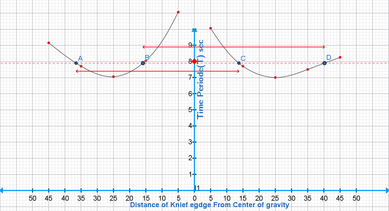
- Take the Y-axis through the middle of the graph paper, with the origin corresponding to the centre of gravity G.
- Represent the distance l of the suspension point from G along the X-axis. Plot the suspension points on one side of G to the right of the Y-axis and those on the opposite side to the left of the Y-axis. Thus, distances measured from G on opposite sides are represented in opposite directions from the origin.
- Represent the corresponding time period T along the Y-axis, using a suitable scale, and plot all the observed points accurately.
- Draw smooth curves through the plotted points on either side of the Y-axis, taking care that the two branches are symmetrical about the Y-axis, within the accuracy of the experimental observations.
- For a selected value of T, draw a horizontal line parallel to the X-axis. It intersects the two branches at the corresponding conjugate suspension points.
- If the distances of the two conjugate suspension points from G are l1 and l2, determine the equivalent length of the compound pendulum from L = l1 + l2. Thus, L is the distance between the two conjugate suspension points.
- Repeat this graphical construction for several values of the time period T and determine the corresponding values of L.
- Calculate L/T2 for each selected period. The values should remain approximately constant over the range of periods.
- Determine the mean value of L/T2 and calculate the acceleration due to gravity using g = 4π2L/T2.
- For each pair of conjugate suspension points, calculate the radius of gyration about the centre of gravity using kG = √[l(L − l)], where l is the distance of either conjugate suspension point from G.
- Calculate kG for several conjugate pairs and determine its mean value.
- To determine the radius of gyration graphically from the minimum-period region, draw the required tangent EF to the two branches of the T versus l graph and determine the minimum time period Tmin corresponding to the point where the tangent intersects the Y-axis.
- At the minimum-period condition, determine the equivalent length Lmin from the corresponding graphical construction. Since Lmin = 2kG, calculate the radius of gyration using kG = Lmin/2.
- Using Tmin and kG, calculate another value of the acceleration due to gravity from g = 4π2(2kG)/Tmin2.
- Compare the value of kG obtained from the conjugate-point method with that obtained from the minimum-period graphical method and determine the mean value.
- Determine the mass M of the bar accurately using a suitable balance.
- Calculate the moment of inertia of the bar about an axis perpendicular to the plane of oscillation and passing through its centre of gravity using IG = MkG2.
- Repeat selected observations to check the consistency and reproducibility of the measurements. Determine the mean values of g, kG, and IG, and estimate the experimental uncertainty.
Procedure (Virtual Experiment)
- Open the simulation in Full Screen mode.
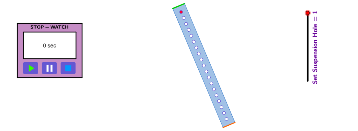
- Use the Set Suspension Hole slider to select the required hole on the knife edge for suspension. Start with Hole No. 1, then proceed with Hole No. 3, Hole No. 5, and so on.
- The centre of mass of the compound pendulum is already displaced through a small angle θ. Click the Play button to release the pendulum, start the oscillations, and activate the stopwatch.
- As soon as the simulation starts, count the number of complete oscillations of the compound pendulum.
- When the pendulum completes the predetermined number of oscillations, click the Pause button to pause the simulation.
- Note the stopwatch reading corresponding to the selected hole number (point of suspension).
- Click the Stop button to reset the simulation and stopwatch before taking the next reading.
- Select the next hole as the point of suspension and repeat the above procedure.
- Record all the observations in the Observation Table provided in the Observations section.
- After entering all the observations, click the Plot Graph button. The graph will be generated using the recorded observation data in the Result and Analysis section.
- From the plotted graph, determine the values of AC and BD, corresponding to l1 and l2, respectively.
- Click the Next button below the graph to open the Freehand Calculation section.
- Perform the required calculations using the Freehand Ink Tool and enter the calculated results in the respective input boxes.
- Click Export PDF to generate and download the completed virtual experiment as a PDF.
Simulation
SimulationObservation Table
Section 06Compound Pendulum Observation Table
Result and Analysis
Section 07Result summary
Use the measured time periods and conjugate suspension points to determine the equivalent length, acceleration due to gravity, radius of gyration, and moment of inertia.
Calculation on freehandTool
g = 4π²L/T²; K = √[l(L − l)]; I = mK²